第二节 入渗条件下土壤水分运动
一、入渗条件下土壤水分运动的半理论半经验公式
入渗条件下土壤水分运动的解析求解有多种方法,现仅对其中较为简单的拉普拉斯变换法、级数法和Green—Ampt模型三种方法进行介绍。
1.拉普拉斯变换法
降雨和灌水入渗是补给农田水分的主要来源。入渗速度、总量和入渗后剖面上土壤含水率的分布,对确定农田水分状况的调节措施有重要意义。兹以地下水埋深较大,剖面土壤含水率均匀分布,地表形成薄水层情况为例,说明入渗条件下土壤水分运动的拉普拉斯变换解析法。
在垂直入渗的情况下,坐标轴z=0取自地表,取z向下为正,位置水头z为负值,一维土壤水运动的基本方程可写成:

如降雨或灌水前剖面上各点初始含水率为θ0,则初始条件为:

在地表有薄水层时,表层含水率等于饱和含水率θs,在z相当大(z→∞)时,含水率不变,即θ=θ0,则边界条件为:

式(1-22)为非线性方程,求解比较困难。为了简化计算,近似地以平均扩散度 代替D(θ),由于
 ,以
,以 代替
代替 ,则式(1-22)变为常系数线性微分方程:

采用拉氏变换求解。经变换后θ的象函数 为:
为:

对式(1-25)中 采用拉氏变换,即

采用分部积分法,设 =du,e-pt=v,u=θ,dv=-pe-ptdt

对式(1-25)右侧进行变换,得:

式(1-25)经变换后,由于仅包含象函数对z的导数,可写成常微分形式:

式(1-24)经变换后,得

式(1-25′)的通解为:

式(1-24′)由于在z→∞时, 为有限值
为有限值 ,为使C1e∞为有限值,C1必须为0,则式(1-24′)可写为:

代入(1-26)式,得象函数 的解为:
的解为:

由拉氏变换逆变换表:

经逆变换后,得

式中: 为补余误差函数。

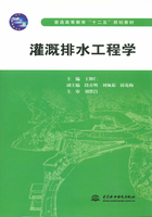
剖面含水率分布可从式(1-26′)求得,如图1-7所示。
地表入渗速度的计算式为:


图1-7 入渗条件下土壤剖面含水率分布图
由于在有水层入渗时,地表处含水率达到饱和,K(θ)=Ks等于土壤饱和时的水力传导度。D(θ)仍采用平均值 ,
, 可自象函数
可自象函数 推求,自式(1-26)

在入渗初期 时,根据拉氏变换原理,相当于
 。
。
查逆变换表:

代入式(1-27),得:

在入渗时间较久时, ,相当于
,相当于 此时
此时 =0,i=Ks,因此,可将式(1-28)作为入渗速度的近似计算式。
在时间t内入渗的总水量I为:

2.级数法及Philip公式
Philip(1957年)利用级数法对入渗问题式(1-22)进行了求解,求得了垂直入渗的级数解:

式中:I(t)为累积入渗量,右端第一项为土壤剖面中土壤水的增加量,第二项为下边界的重力下渗量;K(θi)为初始含水率θi相应的导水率。
作为一种近似,只取级数解中的前二项,即

上式又可表示为

入渗率i(t)相应地为

式(1-30)和式(1-31)便是Philip的入渗公式。习惯上称Philip入渗公式的参数S为吸渗率,称A为稳定入渗率[A=i(∞)]。S和A分别为

在入渗初期,参数S起主要作用,相当于水平吸渗的情况。随着入渗时间的增长,参数A则成为影响入渗的主要因素。
当应用Philip公式解决实际问题时,参数S和A常由现场入渗试验确定。
3.Green—Ampt模型
Green—Ampt模型研究的是初始干燥的土壤在薄层积水时的入渗问题。基本假定是,入渗时存在着明确的水平湿润锋面,将湿润的和未湿润的区域截然分开。也可以说含水率θ的分布呈阶梯状,湿润区为饱和含水率θs,湿润锋前即为初始含水率θi。这种模型又称活塞模型。在上述假定的基础上,利用达西定律,经过适当的简化与推导,可得出Green—Ampt(1911年)入渗公式:

式中:ic=Ks;b=Ks(θs-θi)sf;Ks为饱和导水率;θs为饱和含水率;θi为初始含水率;sf为土壤水吸力。
当入渗时间t达到一定时间以后,I值足够大,则i→ic,故ic也称为稳渗率。当t→0时,I→0,则i→∞。
该公式简单且有一定的物理模型基础,故长期以来受到重视。此公式虽是按均质土壤导出的,但将其应用到非均质土壤,或用于初始含水率分布不均匀的情况,也都获得了较好的结果。Green—Ampt入渗模型应用的首要问题是如何正确地确定参数Ks和sf。
(1)参数Ks的确定。入渗时,地表至湿润锋面之间含水率分布均一的假定,一般不会引起较大的误差,但地表含水率θ0值是较饱和含水率θs为小的某个值。因而入渗公式中(θs-θi)应换为(θ0-θi),Ks应换为K0,显然K0<Ks。Bouwer(1966年)建议取K0=0.5Ks,K0即为稳定入渗率ic,其值可由田间入渗试验测定。
(2)湿润锋面处平均的或有效的基质吸力sf的确定。可采用土壤水吸力s的加权平均值作为sf,即。式中:Kr=K(s)/Ks为相对导水率。

对于Green—Ampt模型,I=(θs-θi)zf,式中zf为地表至湿润锋面的距离,故还可采用Green—Ampt模型推求入渗过程中湿润锋面的位置。
二、入渗条件下土壤水分运动的经验公式
考斯加可夫(А.Н.КОСТЯКОВ)公式、霍顿(Horton)公式和概念模型均为经验公式,形式简单,应用广泛。
1.考斯加可夫公式
考斯加可夫(1932年)入渗公式为:

式中:B和α为取决于土壤及入渗初始条件的经验常数,由试验或实测资料拟合得出,本身无理论意义。此式表示当t→0时,i→∞。而当t→∞时,i→0的情况,只在水平吸渗条件下才可能,垂直入渗的条件显然是不符合的。
2.霍顿(Horton)公式
Horton(1940年)提出的入渗公式是:

式中:i0、ic和β为经验参数。当t→0时,i不是趋于无穷大,而是一有限值i0,可称为初渗率;当t→∞时,i=ic,故ic为稳渗率。β值决定了入渗率由i0减小为ic的速度。
上述各种入渗公式,无论是半理论半经验型的,还是纯经验性的,在一定程度上都反映了入渗规律,因而都有其实用价值。因此,根据实际问题的需要,可选用其中一种公式计算或选用几种公式进行比较。无论采用哪种入渗公式,均应通过现场试验或实测资料分析取得入渗参数。所选用的入渗模型均应得到实践的验证。